2017/09/04

Heat Conduction Equation


This blog is intended to summarize the Heat Conduction Equation and its derived forms in different analyses. Prerequisite to this article is basic knowledge in Heat Transfer and therefore explanation of the used symbols in the equations, as well as explanation of formulas is excluded from this writing.

Heat conduction in a medium is a dimensional process, depending on the number of dimensions in which it acts. It also varies with time, however, based on the assumptions of steady state (when the temperature does not change with time), or unsteady state (transient), one can have two approaches.
The following flowchart is intended to help distinguishing the states and to select the best suited case with formulas provided.

Steady: no change with time at any point,
Transient: variation with time and position.
(Lumped system: variation with time but not with position.)
Figure 1. Conduction main flowchart
In the Steady State Conduction the temperature is independent of the time change. One can further distinguish one dimensional heat transfer, where the temperature change varies only in one direction. We can talk about multiple dimensions as two- and three-dimensions, which are calculated in a different manned.
In case of 1D conduction, the function depends only on the x dimension, therefore the partial derivatives are replaced by ordinary derivatives.

General form of Heat Conduction Equation (HCE), in rectangular coordinates is called: Fourier- Kirchoff equation:
The general HCE equation can be derived into different special forms, depending on the assumptions and the used boundary conditions.

Boundary and initial conditions for HCE:
There are 4 main boundary conditions used or HCE, these are:


  1. Temperature of the surface (TS) at any time is given,
  2. Heat flux (qS) on the boundary at any time is given,
  3. Fluid temperature distribution (Tf) around the system and convective heat transfer (h) between the system and the fluid is given:
  4. Balance of heat fluxes on both sides of the boundary is given, (applied between 2 solids of different thermal conductivity)
Figure 2. Steady State Conduction flowchart

Figure 3. Transient Conduction flowchart


Figure 4. Transient Conduction computation flowchart


References:
·         Yunus A. Cengel – Heat Transfer – A practical approach, second ed., 2003

·         Heat Transfer lecture notes – Maciej Jaworski, Warsaw, 2016

2017/08/15

Hyperbolic and diagonalizable matrices

HOW TO DETERMINE IF THE SYSTEM OF LINEAR EQUATION IS HYPERBOLIC?

When dealing with system of Partial Differential Equations (PDE) one may have to determine if the matrix A, satisfying the equation is whether hyperbolic or not. In order to determine if a system of PDE is hyperbolic, one must determine if the matrix is diagonalizable.

To open full text: click here

Reference: Advanced Computational Fluid Dynamics, Lecture notes - Jacek Rokicki, 2014

2017/05/01

Finite Difference method

In this post, you can see how the analysis of the accuracy of the given finite-difference formula is achieved for a first order derivative case.
In order to solve ODE problems or Partial Differential Equations (PDE) by system of algebraic equations, there are certain methods available. The Finite Difference method is probably the oldest numerical method that is used.
Figure 1. Numerical solution flowchart
It is recommended to choose a uniformly distributed grid size, having the size of X and Y components the same, due to memory limitations.

Suppose that function U(x) is given as such:
Figure 2. Selection of points on a function
One would like to estimate the first derivative of the function U(x) at some point x(j). The value of the neighboring nodes are given: uj = u(xj), uj+1, uj-1, where xj = j*h.
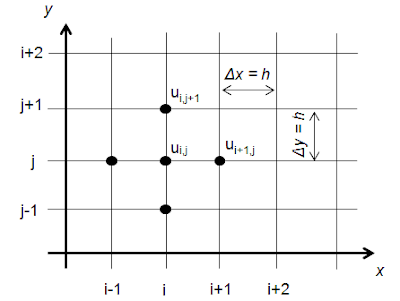
Figure 3. 2D final difference grid
Having a differential equation for a 2D, compressible flow, non-viscous, non-stationary:
One takes the definition of the first derivative:
If the discretization is small enough (Δx), it will approximate the value of the function as:

Similarly to Equation (1.2) one can propose different algebraic formulas for determining the determinant for a given point of the function.
It is important to notice that Equations (1.2) and (1.4) are 1st order accurate, meanwhile (1.5) is 2nd order accurate.
Figure 4. Different approximations
From the above plot, it is clearly visible that out of the 3 different formulas for finding the derivative at a given point Xj, the line that is closest to the tangent point at that point is III. This is the so called central difference and is more accurate that the other, forward difference one. The errors can be determined simply by the Taylor expansion.
Similarly to Equation (1.3) the following algebraic equations can be written:
One can conclude that the finite difference formula has order of accuracy n and is proportional to hn for small values of step size h. The central difference is 2nd order accurate and higher order terms are resulting in lower accuracy, therefore the 2nd order formula works best for calculating ODE-s and PDE-s.
Other method for deriving finite difference formulas (with different accuracy) for a given differential order remains a problem to solve.


To download full text in PDF: click here
Reference: Computational Fluid Dynamics, Lecture notes - Jacek Rokicki, 2014

2017/01/07

How to create Half-Section View in NX Unigraphix - Drafting

Demonstration the problem with Section View
The following blog is describing how the one can create break-out section views for engineering drawings, using Siemens UNIGRAHIX NX software.
I personally find NX Drafting a long, time taking process therefore it's always good to have some tricks handy. (Click on images to obtain full size.)


The problem:

If the one would like to create a half section of an object on different projections, there is a tool called "Section View" which can create a view from any parent drawing view but it will require always to have both views shown.

This can be done by simply clicking at the desired point (with Dynamic Section Line definition) or by creating a sketch for the section line (with Select Existing). This second option requires a sketch that can be created with the "Section Line" option.

However, any of these options will make the section and add the cutting lines, arrows and lettering, which is unwanted. Any half-projection is requiring a different and complex method.→ The question arises, how to make a proper half-section then?


Step-by-step solution:


Simple Assembly

(For the demonstration, a simple composite wall, with integrated sleeve and bolt is assembled. This is just a simple, quick model, no guarantee of correct alignment of elements and dimensions.)


1. Place a top view and a side view.

2. Activate the view that you would like to have half sectioned.


3. Draw a circle/Studio Spline around the area that encloses all the components that you would like to cut in half. Then Finish Sketch.


4. Select Break-Out Section option:


- "Select view for break-out creation": Select the drawing frame of the view where you want the section to be.

- "Define base point - Select object to infer point": In this step, you need to use the other view, and select a point through which the cut will be done on the other view. (in most cases it lies on a symmetry plane or a center of a circle)

- "Define the extrusion vector or continue to accept the default - Select objects to infer vector": You may accept or reverse the vector in which direction the cut will be made. An orange arrow shows this on the view where the base point was selected. If you accept direction, continue with next step without clicking anything here. If not, reverse vector.

- Click on "Select Curve" and "Select break line near start": then you need to select the previously drawn circle or spline curve.

- Click Apply and wait for the half section to be loaded.
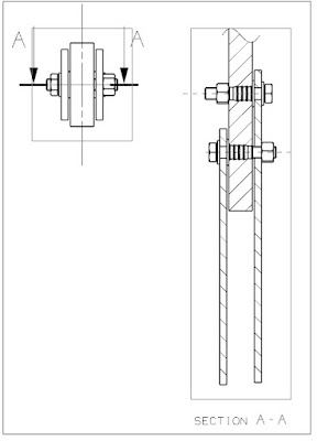
Half-section after Break-Out View

5. Now you can delete the other view that was only needed for selecting the "Base point". This way you can only have one view and not like in the case of Sections with arrows.


Note that after completing a break-out section, no modification is possible. The same is true after deleting the second view, it has to be added again and start the whole process from the beginning.


Next part deals with correcting the view for engineering drawing compatibility. (Here is where your theoretical knowledge comes in, since any CAD software you're using, won't tell you how to do so. You as an engineer/designer need to know the correctness of your drawings!)

Adding and removing hatching on object:


It may seem in some cases that there is no hatching on a surface. If you look carefully, you will find a tiny line that is part of hatching but the distance is too large between the hatching lines. In such case, changing the distance of the hatching lines will solve the issue.


To get rid of hatching where it is not needed:


(e.g. Bolts, pins, washers, shafts should never be hatched.)

Use: Section in View:

- Select View: Drawing frame- Select Object: I recommend right-mouse-clk on the object and "Select from list..." that is hatched and select proper one corresponding to the object. In this case, you will always select the right object, not the one that NX offers first.- Action field: Select "Make Sectioned"- Ok/Apply- Right clk on drawing and update view. Only then you will see the change.


----------------------------------------------
---------------------------------------------------------------------
------
Possible problems that might occur:


According to NX detailed description, the one can check the following things to solve the problem:


  Recommended Actions

  -------------------
    o  Choose Ignore to restore the view to the state it was in
       prior to the update.  This is the DEFAULT action.
    o  Choose Suppress to convert the view to manual update.
    o  Choose Delete to delete the view and all associated objects.

  Possible Corrective Actions

  ---------------------------
    o  Validate and fix the model
    o  Set view to manual update
    o  Set view to reference
    o  Recreate view
    o  Remove view
    o  Suppress view update
    o  Fix invalid section lines
    o  Validate layer settings
    o  Unsuppress suppressed solid bodies
    o  Re-establish section segment associativity in
       Edit Section Line