2015/11/18

When it comes to disaster

During your engineering career you will probably experience the burden of responsibility. Especially when working in the field of aviation, the world of safety regulations, you may have the fear, what if “my aircraft” fails in some way. Have I done those calculations correctly and precisely? Regardless of what you are doing, you must always do your job with full care and attention and make sure that none of the things will cause any incident, failure or worse. An aircraft has many “back-up” systems and lots of redundancy is involved but still there could be human factors, technical malfunctions or sabotage that could lead to disaster.

Recently there has been a Metrojet accident over Egypt, where an Airbus A321-200 aircraft was crashed. The final report of the investigation will most probably determine the causes of this crash therefore we have no right to state anything about it.

What I know so far, is that I was working on that specific aircraft the year before the accident. EI-ETJ is the aircraft registration code, and looking back my notes and photos, I have realized, this is the same aircraft. The aircraft had a complete C-check a year ago and a right engine replacement. Just like all the other planes, it was safely sent back to service from the maintenance hangar for further flights.

There is this strange feeling about the situation, as you feel involved in that plane’s life. Those old seats that were replaced, the old smell from that deck, the cockpit, the engines, the vibration of the whole plane that you felt during its engine test, it’s all a memory. Let’s remember for those who have lost their lives on this aircraft and hope to find out as quickly as possible the causes of this catastrophe.


Reference:

This blog has nothing to do with the airline or any nationality. The pictures are NOT for any further use or for any downloading purposes. The blog is only an engineering point of view into the aircraft industry. Any discussion related to the accident that may be insulting will be removed.

2015/11/08

Boeing 787-8, the Dreamliner


The Dreamliner for me is still a wonder, and engineering masterpiece. I’ve recently came across the following picture posted by LOT – Polish Airline’s facebook site, which just caught my attention. (this is not an advert)


Have a look at how this 'beauty' is made up or what structural elements an aviation aficionado sees.

Thank you for the photo permission and credit to Marek Kwasowski.

2015/10/19

Weather forecasting with the help of CFD

In this blog, I am intending to present a basic equation of Fluid Mechanics, then give some related views on weather forecasting science with a help of a useful and versatile website. Finally give some hints about METAR, the meteorological "code" used by pilots.

For the sake of simplicity, let's introduce the following equation to lose 90% of the readers of this blog.

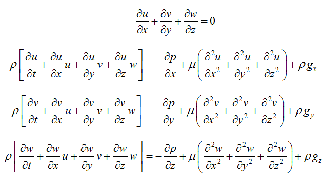
The Navier-Stokes equation for compressible fluid
It this form, the body force f has been decomposed, but the mass conservation, equation of state and equation for the conservation of energy is needed.

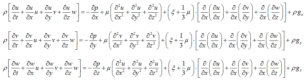
To write it in an even more general form:
Which written in an expanded form:
where: 


To solve the above equation, one needs to know initial conditions, such as pressure – p(r,t) , temperature – T(r,t) and velocity – V(r,t), which are usually provided.


(more about the equation in another blog: Navier-Stokes 3D fully expanded form)

Weather forecasting is basically the simulation of time-dependent phenomena, the solution of the N-S equation with the help of the known initial conditions. The initial conditions can be density, temperature, (wind) velocity and pressure. With the help of atmospheric models, one can compute meteorological information for future times at given locations and altitudes. The measures are taken from the meteorological ground stations, weather balloons and satellites as well.
Wind forecasting at surface level (Source: www.windyty.com)
Many websites provide such weather information but probably one of the best looking and advantageous is: windyty.com


The site allows you to display the streamlines of wind, temperature profiles, clouds, waves, snow and pressure information about given altitudes. Even more, by clicking to any location, the one can find detailed forecast for that location. Many more info is displayed, as the site is connected to the latest METAR-s measured at certain airports.


What exactly is METAR and how it is used in aviation?
The first thing which might be new on the above picture, under the 'Warsaw' text, is: 'EPWA', which is the ICAO code for Chopin Airport. (Each airport has such identification code but this may be the topic of another blog.) Coming back to the METAR, which is a line of code, made at each meteorological stations on some airports. This is the code that pilots are receiving and this is set into the flight instruments. Looking at EPWA's METAR code:


EPWA 182130Z 23003KT 200V270 6000 -RA BKN049 08/07 Q1017 NOSIG

  1. EPWA
    It starts with the already defines ICAO code of the airport.
  2. 182130Z
    Then follows the day and time: 18th of the month, at 21:30, Z - "zulu", meaning the local time when the measurement was made.
  3. 23003KT 200V270
    This is the average of the surface winds in 10 minute intervals.
    The first three digits are showing the direction of the wind, which in this case is 230° and the next two digits are the velocity, that is 4 knots (KT). MPS - if given in m/s, KMH - if given in km/h-s. (If the wind velocity is greater than 100 knots, it'll be 3-digits long.)
    If during the 10 minutes interval the direction of the wind has changed 60° or more and the wind's velocity is greater than 6 km/h (3kt), then the two boundary directions has to be displayed, in clockwise direction. The letter V (varied) is used to separate these directions. In our case; the wind has changed direction between 200°and 270°.
  4. 6000
    Horizontal visibility given in meters.
  5. -RA
    This section is for the actual weather conditions, given in codes. RA - rain, the negative sign means light rain.
  6. BKN049
    This field is dedicated to the clouds. The first part is the quantity of clouds, given by the numbering system following it. So 08/07 belongs to the BKN - Broken clouds category. The next three digits: 049 is the cloud base altitude in feet: at 4900feet. (
  7. 08/07
    The first two digits are the temperature, the next two are the dew point 
    in degrees.
  8. Q1017
    QNH - 
    barometric pressure adjusted to sea level, given in hectopascals: 1017hPa.
    (1013 mbar = 29.92 inHg = 760 Hgmm = 14.69 PSI)
  9. NOSIG
    Meaning no significant change is expected.
METARs for a given location (Source: windyty.com)

This code can of course change in any conditions, can have more terms, more information, depending on the weather itself. In this blog, I only wanted to present the idea behind it, of course this simple code "METAR" could be a whole course on how to write, interpret it and so on. The website has the feature that it encodes this METAR into a user friendly code, making it available to read by anyone.


I hope this blog helped to understand the compressible N-S equation and gave a useful link to weather forecasting in a fun way. Start exploring for such beautiful and colorful maps.
Pressure at 10km altitude (Source: windity.com)

Resources:
  • John D. Anderson Jr. - Fundamentals of Aerodynamics, Fourth edition, Chapter 15. pp., 2007
  • https://en.wikipedia.org/wiki/Atmospheric_model
  • https://www.windyty.com
  • CFD lectures - dr Jacek Rokicki

2015/10/17

Difference between solids and liquids

Have you ever been asked to define how solids are different from liquids? Is it the density or rather the pressure difference acting on them? Maybe whether the two matters are compressible? Not quite...

The most important difference between solids and liquids, from fluid mechanical point of view, is in its' stresses
When talking about solids; the stresses are depending on the deformation. If one is applying force to an object, it'll have inner stresses generated inside the molecules. If the same force would be applied to a liquid, it will probably not generate anything, and will not affect much the state. In case of liquids, the different source of stresses are achieved by the velocity of deformation.

One can write the constitutive equation, for a Newtonian fluid:
Where: T - stress tensor, I - identity matrix, μ - viscosity term
D - divergence of velocity / deformation velocity tensor, expressed as:
The reason, why liquids flow lies in the above equation. The stress does not depend on deformation but depends on deformation of  velocity. In all kinds of fluids (except for superfluids), any change in deformation increases the viscous forces within the matter, due to the friction between the adjacent particles. The stress state tensor is describing these stress changes at any point of the fluid domain.


Resources:
  • https://en.wikipedia.org/wiki/Strain_rate_tensor
  • http://www.zmescience.com/research/shear-difference-liquid-solid-0549123/
  • Computational Fluid Dynamics lecture - dr Jacek Rokicki

2015/06/25

Lifting-line model of a finite-span wing (Wingtip vortices)

This blog is meant to give a basic definition about the wingtip vortices and to give a sense of the lifting-line model of a finite-span wing.

Tip vortices and down-wash generated behind an airplane are shown.


You may see on the pictures the tip vortices that are visualized by the clouds. On the second picture, there's a plane shortly after take-off, very high angle of attach, so there is a very huge lifting force of course, and you can see the vortices generated and their mixing in the air with the upstream and downstream flows.

Another picture of an agriculture airplane of which's tip vortex is visualized. Significant is the size of the vortex and its huge intensity, compared to the size of the aircraft.

The following figure is showing the visualization of flow past a rectangular wing. Due to the pressure difference between the upper part and the lower part and the fact that the wing has a finite span, there will be a certain tendency of the air to flow from the higher pressure to the lower pressure part. We have counter rotation vortices at the ends of the wing. If I have a streamline at the bottom surface then near the wing tip it’ll be deflected as it’s indicted with the dashed line. On the other side, on the suction side, the streamlines will be deflected towards the fuselage.

Initially it was very difficult to create a realistic geometric model of this type of the vertical wake so they came up with an idea; instead of taking this spiral folding, make our “vortical” wake behind the airfoil completely flat. It doesn’t mean that there will be no vorticity. It means that the self-induction is completely neglected and the vertical flow is assumed to be completely flat. It’s of course not true but we can build the model of the wing.

Flow past a wing is modeled by the superposition of the uniform free stream and the velocity induced by a plane vortex sheet “pretending” to be the cortex wave behind the wing.

The idea of Prandtl was that; imagine if we have infinitely many vortex lines, of which each of them has such shape as shown on the figure:
(It extends from infinity along what is called a lifting line, which completely replaces the wing and goes back to infinity.) These infinitely many vortex lines are overlapping along the lifting line. Beyond the lifting line they form a vortex sheet which is a flow-stream with distributed vorticity. Where they overlap, they create an infinitesimal contribution to "gamma" – dГ, to the total vorticity – Г(y). Since they overlap, Г will have a symmetrical distribution. Each of these lines is called a horseshoe vortex.
Rohács József, Gausz - BME - Aerodinamika page 78.Figure 4.4.
In other words, the vortex sheet behind the wing is “woven” from continuum of infinitesimally weak horseshoe vortices. These vortices are “attached” to the lifting line leading to a continuous distribution of circulation along the wing span.

We’d like to calculate the velocity, induced by this vortex sheet along these lines. Each of these horseshoe vortices induces a certain velocity distribution along y line, which is completely vertical, which means that higher velocity is in z direction. Next it is assumed that each infinitely thin slice of the wing generates the (differential) contribution to the total aerodynamic force as it were a 2D airfoil. Each slice “senses” its individual direction of “free stream”, which results from the real free stream vector V and the vertical (normal to the vortex sheet) velocity induces at the lifting line in the point corresponding to the position of the wing slice.


References:

Photos: Airliners.net, NASA.gov

  • Timo Harsch - Airbus A340-642 ZS-SNG
  • Colin Hollywood Photography - Boeing 777-F6N B-2083
  • Helmut Schnichels - Airbus A380-842 VH-OQA 
  • Aerodynamics lecture, by Jacek Szumbarski, Warsaw University of Technology
  • Rohács József, Gausz - BME - Aerodinamika jegyzet, page 78. figure 4.4.

2015/06/22

Navier-Stokes equation for 3D compressible and incompressible flows

In this blog I would like to present the general form of the Navier-Stokes equation for both incompressible and compressible flows. As in most textbooks you may not find the fully expanded forms in 3D, here you have them all collected. For the first look, it might scare you but after breaking it down, it’s all simple. 

Incompressible flow:
  • Frame invariant form:
  • Dimensional form:
The subscripts imply differentiation with respect to the variables. Primes (‘) indicate that the unknowns are dimensional. The system of equations are solvable, since there are 4 equations and 4 unknowns: 

Fully expanded form to 3D coordinates:

Compressible flow:


  • Frame invariant form:

  • Fully expanded form to 3D coordinates:


Resource:
  • Aerodynamics for Engineering Students, Sixth Edition, E.L. Houghton, (etc.)

The equations were typed into Microsoft Office, unfortunately blogger.com does not have a possibility to type equations so I had to make screenshots of them. You may use them freely as you wish. Beware of the fact that there might be minor mistakes in the formulas, although I checked them several times.

2015/06/20

Engineering approach to prediction of the laminar-turbulent transition in the boundary layer (e^N method)

The most popular and effective engineering methods of transition predictions are based on the idea of the e^N method.

Since the amplification is of the exponential form, the corresponding amplification factor with distribution of x will look like as given on the Figure. Note that starting from the maximum point, this Tollmien-Schlichting wave is not amplified anymore and it starts to be diminishing. But this is just one frequency. If I choose any other frequency, I can have such lines that’ll rise later. We have infinite number of Tollmien-Schlichting waves with different frequencies and we have individual curve of each of them.

The idea of e^N method for transition prediction was published by Van Ingen in 1956.
The above formula describes the cumulative amplitude growth that is determined for a bunch of modes with different frequencies. One can obtain as a result a family of lines, showing how the amplification factor of each mode grows downstream the boundary layer (BL). In principle, if I have a boundary layer, then in BL we have an excitation of all possible frequencies. Then, one can define the envelope for this family, which is a line effectively parametrized by the frequency. (see Figure) 

We assume that the actual amplification of disturbances in the BL will be inside this envelope. So if I choose a line, which sort of has all this infinitely many lines underneath, then I will be on the same side. So if I can calculate this envelope line, which goes on the top of all individual lines, I’ll have sort of a border of a maximum possible local amplification that may in principle happen in any cross section on the TBL. The hypothesis behind it also says that the actual transition point will be when this envelope will reach a certain value of this logarithm. For example, when the flow is in a very calm atmosphere, where the lever of turbulence outside the BL is very-very small, then the BL will survive without being stabilized such amplification and a local amplification up to say 9 orders of magnitude of initial disturbance. So this logarithm is 9.
But if the external disturbance field will be much higher, then that means that from the very beginning the disturbances are large, so it’s enough e.g. to amplify them by 4th order of magnitude, or maybe 5th order of magnitude, before they actually cause a transition to the TBL.

Physically the idea is primitive but surprisingly it works very well. Over the years, people gained a huge experience in manipulating this amplification factor and e.g. those Aerodynamists who use for aerodynamic design software like Xfoil, they know very well which amplification factor with this e^N criterion to choose. Dependently on the different conditions for which this or another airfoil is actually designed. If it’s designed for a glider, which supposed to fly in a very calm atmosphere, that’s the situation it supposed to get its best of its performance, then the one should choose this very-very small. The level of this is not about the level of external atmosphere but it’s also about the quality of the surface of the wing. If it’s very well polished, like a “glass”, which is most typical for modern gliders then this number can reach ever 11, for the measure of transition. But if we have something like a small wind turbine, small like, someone puts it on a farm, there is send around, there are insects on it, probably bird was hit by the blade, there is feather here and there on it, so the quality is very-very bad, it could be even lowered to around 4, especially if this contamination of the surface is close to the leading edge.

There is another important issue. If you have an airfoil and you’re worrying about making it dirty, then if this dirtiness is in front, near the leading edge, it’s really dangerous. If it’s far away, near the trailing edge, it’s not dangerous. This is pretty obvious. Initially the thickness of the BL is very-very small, meaning that even a small obstacle from the point of view of the laminar BL is huge. The same obstacle, when flown to the airfoil somewhere near the trailing edge, for the BL which is now 10 times thicker, is simply less sensitive.


Reference:
  • Aerodynamics lecture, by Jacek Szumbarski, Warsaw University of Technology

2015/06/05

Changes of the slope of the lifting force characteristic CL=CL(α)

How the slope of the lifting force characteristic CL = CL (α) changes with increasing thickness and camber of the airfoil according to the potential flow theory and according to the thin airfoil theory?

Potential flow theory:

According to the potential flow theory, the slope of the lift force characteristic for the Joukovsky’s non-symmetrical airfoil with zero thickness (ε = 0) is expressed by the approximate formula:
where f is the camber ratio (ratio between the maximal deflection of the mean camber line and the chord of the airfoil).
The small correction is proportional to the square of the camber. The thicker the profile of the airfoil, the more the slope of CL = CL (α) is increased.

The formula for the lift force coefficient can be written as follows:
where β is negative and corresponds to zero lift condition.
The deflection of the airfoil (AoA) leads to the vertical shift in the characteristic CL = CL (α) curve, as the equation is α dependent.

Thin airfoil theory:

The slope of the lift force characteristic CL = CL (α) is equal:
From which it can be clearly seen that the slope does not depend on the airfoil camber. It does not include also the correction as it was in the potential flow theory.

The formula for the lift force coefficient can be written as follows:
where
 is the negative angle of attack at which the camber airfoil is not producing any lift.
Summarizing it: